4. Choosing the learning paradigm#
Note
This blog post by Scott Login will help you better understand the memory requirements.
Warning
To run this notebook, you will need access to at least one GPU. The results that are printed were obtained using a single A100 graphic card with 80 GB of memory. Note that even using such a powerful GPU took the notebook more than 10 hours to complete.
This book aims to illustrate with a practical example how to decide which learning paradigm is better for each application. To demonstrate the process, we will extract some information about chemical reactions from paragraphs of text.
4.1. First steps#
Choosing the learning paradigm should begin by trying some leading general-purpose LLM. For this practical case, the first model to test is the recent Llama-3 8B model with zero and one-shot prompts.
We will start by importing all the packages needed.
import matextract  # noqa: F401

import json

import torch
from datasets import (
    load_dataset,
    Dataset,
)
from transformers import (
    AutoModelForCausalLM,
    AutoTokenizer,
    BitsAndBytesConfig,
    TrainingArguments,
    pipeline,
)
from transformers.pipelines.pt_utils import KeyDataset
from peft import (
    LoraConfig,
)
from trl import (
    SFTTrainer,
    DataCollatorForCompletionOnlyLM,
)
from evaluate import load
from litellm import completion
from statistics import mean
import numpy as np
import matplotlib.pyplot as plt
To continue, we will allow LiteLLM to cache requests made to LLM-APIs. Additionally, we will import all environment variables.
4.2. First model and dataset#
As starting model, we will try the Llama-3 8B model. We will call this model through the Groq API, which allows performing fast inference with several open-source models.
base_model = "groq/llama3-8b-8192"
The dataset used in this tutorial is the one used in Ai et al. [2024] recent work, which contains data about chemical reactions text-mined from United States patents. The dataset, the so-called USPTO-ORD-100K dataset, contains 100K reaction procedure-ORD schema pairs. To make easier the download of the data, we created a Hugging Face dataset, that will be used here, as well in the case study about Collecting data for reactions procedures.
test_dataset = load_dataset(
    "MrtinoRG/USPTO-ORD-100K", data_files="test.json", split="train"
)
test_dataset = test_dataset.shuffle(seed=42).select(range(100))
test_dataset
Downloading readme: 100%|██████████| 24.0/24.0 [00:00<00:00, 35.2kB/s]
Downloading data: 100%|██████████| 29.8M/29.8M [00:02<00:00, 14.0MB/s]
Generating train split: 10000 examples [00:00, 33384.31 examples/s]
Dataset({
    features: ['instruction', 'output'],
    num_rows: 100
})
test_dataset[0]
{'instruction': 'Below is a description of an organic reaction. Extract information from it to an ORD JSON record.\n\n### Procedure:\nThe procedure of Example 1a) was repeated, except that 743 mg of 4-nitrobenzyl (1R,3R,5R,6S)-6-((1R)-1-hydroxyethyl)-1-methyl-2-oxo-1-carbapenam-3-carboxylate and 1.06 g 2-(tri-n-butylstannyl)-7-trifluoromethylthioimidazo[5,1-b]thiazole were used as the starting compounds. Thus, 172 mg of 4-nitrobenzyl (1S,5R,6S)-6-((1R)-1-hydroxyethyl)-1-methyl-2-(7-trifluoromethylthioimidazo[5,1-b]thiazol-2-yl)-1-carbapen-2-em-3-carboxylate was prepared.\n\n### ORD JSON:\n',
 'output': '{"inputs": {"m1": {"components": [{"identifiers": [{"type": "NAME", "value": "4-nitrobenzyl (1R,3R,5R,6S)-6-((1R)-1-hydroxyethyl)-1-methyl-2-oxo-1-carbapenam-3-carboxylate"}], "amount": {"mass": {"value": 743.0, "units": "MILLIGRAM"}}, "reaction_role": "REACTANT"}]}, "m2": {"components": [{"identifiers": [{"type": "NAME", "value": "2-(tri-n-butylstannyl)-7-trifluoromethylthioimidazo[5,1-b]thiazole"}], "amount": {"mass": {"value": 1.06, "units": "GRAM"}}, "reaction_role": "REACTANT"}]}}, "conditions": {"conditions_are_dynamic": true}, "outcomes": [{"products": [{"identifiers": [{"type": "NAME", "value": "4-nitrobenzyl (1S,5R,6S)-6-((1R)-1-hydroxyethyl)-1-methyl-2-(7-trifluoromethylthioimidazo[5,1-b]thiazol-2-yl)-1-carbapen-2-em-3-carboxylate"}], "measurements": [{"type": "AMOUNT", "details": "MASS", "amount": {"mass": {"value": 172.0, "units": "MILLIGRAM"}}}], "reaction_role": "PRODUCT"}]}]}'}
This dataset is very big. Therefore, we will only take 100 samples from the test set used in the article mentioned above for our test set.
4.3. Prompt and inference#
We define a simple prompt template. The prompt contains a simple system part (named PREFIX) where the role and task of the model are defined, as well as the example used only for the one-shot prompt. Additionally, the prompt has a user prompt where the reaction instruction will be provided.
PREFIX = """You are a helpful scientific assistant. Your task is to extract information about organic reactions. {shot}"""
SUFFIX = """\n\n{sample}\n\n"""
SHOT = """
One example is provided to you to show how to perform the task:

### Procedure:\nA suspension of 8 g of the product of Example 7 and 0.4 g of DABCO in 90 ml of xylenes were heated under N2 at 130\u00b0-135\u00b0 C. while 1.8 ml of phosgene was added portionwise at a rate to maintain a reflux temperature of about 130\u00b0-135\u00b0 C. The mixture was refluxed an additional two hours, cooled under N2 to room temperature, filtered, and the filtrate was concentrated in vacuo to yield 6.9 g of the subject compound as a crude oil.\n\n
### ORD JSON:\n{\"inputs\": {\"m1_m2_m4\": {\"components\": [{\"identifiers\": [{\"type\": \"NAME\", \"value\": \"product\"}], \"amount\": {\"mass\": {\"value\": 8.0, \"units\": \"GRAM\"}}, \"reaction_role\": \"REACTANT\"}, {\"identifiers\": [{\"type\": \"NAME\", \"value\": \"DABCO\"}], \"amount\": {\"mass\": {\"value\": 0.4, \"units\": \"GRAM\"}}, \"reaction_role\": \"REACTANT\"}, {\"identifiers\": [{\"type\": \"NAME\", \"value\": \"xylenes\"}], \"amount\": {\"volume\": {\"value\": 90.0, \"units\": \"MILLILITER\"}}, \"reaction_role\": \"SOLVENT\"}]}, \"m3\": {\"components\": [{\"identifiers\": [{\"type\": \"NAME\", \"value\": \"phosgene\"}], \"amount\": {\"volume\": {\"value\": 1.8, \"units\": \"MILLILITER\"}}, \"reaction_role\": \"REACTANT\"}]}}, \"conditions\": {\"temperature\": {\"control\": {\"type\": \"AMBIENT\"}}, \"conditions_are_dynamic\": true}, \"workups\": [{\"type\": \"ADDITION\", \"details\": \"was added portionwise at a rate\"}, {\"type\": \"TEMPERATURE\", \"details\": \"to maintain a reflux temperature of about 130\\u00b0-135\\u00b0 C\"}, {\"type\": \"TEMPERATURE\", \"details\": \"The mixture was refluxed an additional two hours\", \"duration\": {\"value\": 2.0, \"units\": \"HOUR\"}}, {\"type\": \"FILTRATION\", \"details\": \"filtered\"}, {\"type\": \"CONCENTRATION\", \"details\": \"the filtrate was concentrated in vacuo\"}], \"outcomes\": [{\"products\": [{\"identifiers\": [{\"type\": \"NAME\", \"value\": \"subject compound\"}], \"measurements\": [{\"type\": \"AMOUNT\", \"details\": \"MASS\", \"amount\": {\"mass\": {\"value\": 6.9, \"units\": \"GRAM\"}}}], \"reaction_role\": \"PRODUCT\"}]}]}
\n
"""
To continue, we loop all over the dataset two times, one for each type of prompt (zero- and one-shot). For each dataset sample, we format the prompt to include the procedure-output schema pairs using the template defined in the previous cell. In addition, we also predict using the model and store those predictions for future evaluation.
shots = ["0-shot", "1-shot"]
results_llama = {}

# Start by looping over the shots
for s in shots:
    predictions = []
    references = []

    # Loop over all the samples of the dataset
    for t in test_dataset:
        instruction = t["instruction"]
        output = t["output"]
        # Format the prompt
        if s == "0-shot":
            shot = ""
        else:
            shot = SHOT
        system = PREFIX.format(shot=shot)
        user = SUFFIX.format(sample=instruction)
        prompt = [
            {"role": "system", "content": system},
            {"role": "user", "content": user},
        ]
        # Do the completion using Groq API through LiteLLM
        pred = (
            completion(
                model=base_model,
                messages=prompt,
                caching=True,
                temperature=0,
            )
            .choices[0]
            .message.content
        )
        # Save the predictions and the references for later evaluation
        references.append(output)
        predictions.append(pred)

    results_llama[s] = {
        "predictions": predictions,
        "references": references,
    }
After generating the predictions, it’s essential to evaluate them. We will initially use the BERTScore for a simple evaluation, as it provides precision, recall, and F\(_1\) scores based on similarity measures. However, for a complex schema like the one we are predicting, more robust evaluation methods should be utilized.
Notes about BERTScore
BERTScore [Zhang et al., 2020] is an evaluation method that proceeds by calculating the similarity of the candidate text with the reference. This similarity is calculated as a sum of cosine similarities token by token. To produce the embeddings for this similarity calculation, in the original article, they used the BERT model’s embeddings. However, for our case we will be using the embeddings from the DistilBERT model [Sanh et al., 2020], which achieves 97% of the original BERT model language understanding while only being 40% the size of BERT original model.
bertscore = load("bertscore")
shots = ["0-shot", "1-shot"]

# Start by looping over the shots
for s in shots:
    predictions = results_llama[s]["predictions"]
    references = results_llama[s]["references"]

    results_ = bertscore.compute(
        predictions=predictions,
        references=references,
        model_type="distilbert-base-uncased",
    )

    results_llama[s].update(
        {
            "precision": mean(results_["precision"]),
            "recall": mean(results_["recall"]),
            "f1_scores": mean(results_["f1"]),
        }
    )
Results for the 0-shot prompt
	Precision: 0.865
	Recall: 0.8918
	F1-Score: 0.8781

Results for the 1-shot prompt
	Precision: 0.9392
	Recall: 0.9553
	F1-Score: 0.9471
The results are very good, especially with the one-shot prompt. However, we are going to try a different model, a closed-source model, to compare.
4.4. Another model, closed-source this time#
The second model we will use is the newer OpenAI, GPT-4o. Doing this allows us to compare open- and closed-source models.
The procedure and code are exactly the same as for the previous case; the only difference is to define a different model.
base_model = "gpt-4o"
And we obtain the completions using both prompts for all the test samples.
results_openai = {}
shots = ["0-shot", "1-shot"]

# Start by looping over the shots
for s in shots:
    predictions = []
    references = []

    # Loop over all the samples of the dataset
    for t in test_dataset:
        instruction = t["instruction"]
        output = t["output"]
        # Format the prompt following OpenAI's prompting guidelines
        if s == "0-shot":
            shot = ""
        else:
            shot = SHOT
        system = PREFIX.format(shot=shot)
        user = SUFFIX.format(sample=instruction)
        prompt = [
            {"role": "system", "content": system},
            {"role": "user", "content": user},
        ]
        # Do the completion using Groq API through LiteLLM
        pred = (
            completion(
                model=base_model,
                messages=prompt,
                caching=True,
                temperature=0,
            )
            .choices[0]
            .message.content
        )
        # Remove some residual stuff in the json output by the model.
        if "```json" in pred:
            pred = pred.replace("```json\n", "")
            pred = pred.replace("```", "")

        # Save the predictions and the references for later evaluation
        references.append(output)
        predictions.append(pred)

    results_openai[s] = {
        "predictions": predictions,
        "references": references,
    }
Finally, we evaluate again using BERTScore.
for s in shots:
    predictions = results_openai[s]["predictions"]
    references = results_openai[s]["references"]

    results_ = bertscore.compute(
        predictions=predictions,
        references=references,
        model_type="distilbert-base-uncased",
    )

    results_openai[s].update(
        {
            "precision": mean(results_["precision"]),
            "recall": mean(results_["recall"]),
            "f1_scores": mean(results_["f1"]),
        }
    )
Results for the 0-shot prompt
	Precision: 0.8949
	Recall: 0.9093
	F1-Score: 0.9019

Results for the 1-shot prompt
	Precision: 0.9545
	Recall: 0.9619
	F1-Score: 0.9581
The results with this GPT-4o model are excellent, improving slightly on the ones obtained with the Llama-3 8B base model. However, we are going to try to improve these results further by fine-tuning the Llama-3 8B model.
Self-verification
For specific cases, self-correction or self-verification seems to be a plausible option to improve results.[Stechly et al., 2024] This technique consists of iteratively prompting the model to verify the correctness of its response. However, this technique is not always applicable, and the results are not always improved.[Kambhampati et al., 2024]
4.5. Fine-tuning#
As the final step, we will fine-tune the Llama-3 8B using data similar to the one we used above.
We will use packages built by HuggingFace to do the fine-tuning.
First, we define the base model we will use and the path of the dataset.
# Model
base_model = "meta-llama/Meta-Llama-3-8B-Instruct"
Caution
It is important to include the HF_token in the .env file. When we created this notebook, the model we will fine-tune (Llama3-8B) was only available after an access request.
The next step is to load the dataset for the fine-tuning. For that, similar to the testing of the previous models, we will use the dataset used by Ai et al. [2024], but for this case, we will use their train dataset. Since this is a quick demonstration, we will only take 5000 samples.
dataset = load_dataset(
    "MrtinoRG/USPTO-ORD-100K", data_files="train.json", split="train"
)
dataset = dataset.shuffle(seed=42).select(
    range(5000)
)  # Only use 5000 samples for quick demo
dataset = dataset.train_test_split(
    test_size=0.1, seed=42
)  # We define 90-10 % training-evaluation splits.
dataset
Downloading data: 100%|██████████| 239M/239M [00:07<00:00, 33.3MB/s]
Generating train split: 80000 examples [00:02, 32150.28 examples/s]
DatasetDict({
    train: Dataset({
        features: ['instruction', 'output'],
        num_rows: 4500
    })
    test: Dataset({
        features: ['instruction', 'output'],
        num_rows: 500
    })
})
Then, we define the method to fine-tune the model. For this fine-tuning, we will use the popular QLoRA method. QLoRA [Dettmers et al., 2023] is an efficient approach that reduces memory usage during fine-tuning while preserving full fine-tuning task performance.
Notes about QLoRA configuration
load_in_4bit=True: loads the model using the 4-bit quantization.bnb_4bit_quant_type="nf4": quantizes following the nf4 method, using a novel datatypenf4(4-bit Normal Float) that is optimized for normally distributed data [Dettmers et al., 2022].bnb_4bit_use_double_quant=True: activate nested quantization for 4-bit base models.bnb_4bit_compute_dtype=torch.bfloat16: Compute dtype for 4-bit base models.
# QLoRA configuration
bnb_config = BitsAndBytesConfig(
    load_in_4bit=True,
    bnb_4bit_quant_type="nf4",  # fp4 or nf4
    bnb_4bit_use_double_quant=True,
    bnb_4bit_compute_dtype=torch.bfloat16,
)
Notes about LoRA configuration
r: The rank of the updated matrices, expressed as integer, meaning that the adaptor that is build in top of the model to improved will be made by matrices of rank 32. Lower rank results in smaller update matrices with fewer trainable parameters that can not be enough to capture the diverse data during the training. On the other hand, higher ranks may lead to overfitting. This rank is a hyperparameter that needs to be optimized.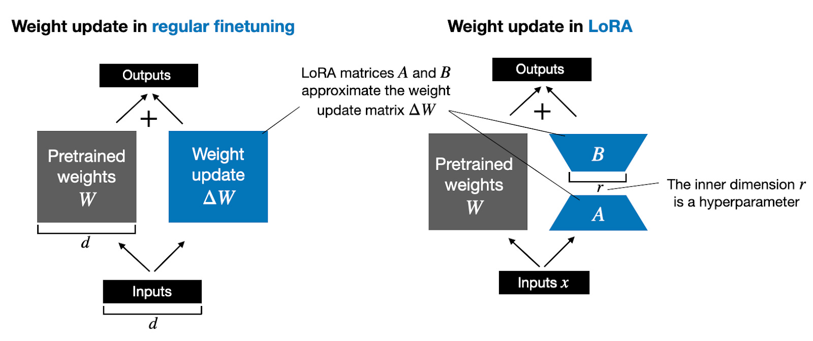
Fig. 4.1 Figure illustrating LoRA rank extracted from a blog post by Sebastian Raschka. Note that lower is the rank, lower is the dimension of the AB matrix multiplication, thus reducing the cost.#
lora_alpha: LoRA scaling factor. It changes how the adaptation layer’s weights affect the base model’s.lora_dropout: Dropout is a regularization technique where a proportion of neurons (or parameters) are randomly “dropped out” or turned off during training to prevent overfitting.bias: Specifies if the bias parameters should be trained. Can be ‘none’, ‘all’ or ‘lora_only’.task_type: Task to perform, “Causal LM”: Causal language modeling.
The Unsloth documentation provides a detailed description of the LoRA parameters and how each impacts the training.
peft_config = LoraConfig(
    r=32,
    lora_alpha=64,
    lora_dropout=0.1,
    bias="none",
    task_type="CAUSAL_LM",
)
Before training, we define the tokenizer and the model for fine-tuning, set the training arguments, and initialize the trainer.
# Load tokenizer
tokenizer = AutoTokenizer.from_pretrained(base_model)  # Define the tokenizer
tokenizer.pad_token = tokenizer.eos_token
tokenizer.padding_side = "left"  # Where the "pad_token" is placed

# Model config
model = AutoModelForCausalLM.from_pretrained(
    base_model,  # Model that we are going to fine-tune
    quantization_config=bnb_config,  # QLoRA config defined above
    device_map="auto",  # Where the model is trained, set device_map="auto" loads a model onto available GPUs first.
)
Caution with the tokenizer
If strange behavior is observed during the fine-tuning, it can be helpful to decode the inference data just before it is passed to the model. Maybe some unexpected tokens are being produced.
Notes about the training arguments
learning_rate: the learning rate is a hyperparameter that sets how the training algorithm updates the values of the weights.Batch size: it is the number of samples used in one forward and backward pass through the network. Ideally, we would like to increase this number so the fine-tuning will be faster. The problem is that for higher batch number, more GPU memory is needed. For example, for training the model used in this demonstration using the exact same configuration but with a default token length (1024 tokens), with 40 GB VRAM GPU, the maximum batch number is 2. Using 80 GB VRAM GPU, the batch size can be increased to 4.
per_device_train_batch_size: batch size for the training.per_device_eval_batch_size: batch size for the evaluation.
gradient_accumulation_steps: number of accumulated gradients over each batch. Gradient accumulation is a technique that simulates a larger batch size and it is very related to the batch size, since it also allows reducing the computation time. However, contrary to the batch size, during the gradient accumulation the weights of the model are not updated during each forward and backward pass, but gradients are accumulated from multiple small batches before performing the update. Thus, setting a highergradient_accumulation_stepscan help to accelerate the training when increasing the batch size is not possible due to VRAM impediments.optim: optimizer used. The main role of the optimizer is to minimize the loss function. Thepaged_adamw_32bitis the well-known AdamW optimizer. AdamW optimization is a stochastic gradient descent method [Loshchilov and Hutter, 2019].num_train_epochs: number of times that the model goes through each sample during the training. A larger number might lead to the best training results or to overfitting. A lower number might give a model that does not work as expected at all.fp16andbf16: these parameters help to achieve mixed precision training, which is a technique that aims to optimize the computational efficiency of training models by utilizing lower-precision numerical formats for certain variables. For fine-tuning, the choice of both parameters depends mainly on the configuration used during the training, i.e. Llama3 models were trained usingbf16so using the same precision configuration for fine-tuning is recommended. In addition to the Hugging Face documentation, there are some compiled spreadsheets with detailed information about the training configuration for some of the open source models.logging_steps: when the logging is done.evaluation_strategy: the evaluation strategy to adopt during training. The most used is ‘steps’ meaning that the evaluation is done after a certain number of training steps.eval_steps: define in which steps the evaluation is done.max_grad_norm: maximum gradient norm (for gradient clipping). Gradient clipping is a method where the error derivative is changed or clipped to a threshold during backward propagation through the network, and using the clipped gradients to update the weights.warmup_steps: number of steps used for a linear warm-up from 0 tolearning_rate. The warm-up helps to stabilize the optimization process and prevent divergence.warmup_ratio: ratio of total training steps used for the linear warm-up.group_by_length: whether to group together samples of roughly the same length in the training dataset (to minimize padding applied and be more efficient). Only useful if applying dynamic padding.lr_scheduler_type: describes the decay of the learning rate during the training.output_dir: directory to safe the report of the training process.save_strategy: what we want to save during the training. Set it to “no” to only safe the final model.
Fig. 4.2 Shape of the “cosine”
lr_scheduler_typeoption.#
# Define the different hyperparameters and arguments for the fine-tuning
training_arguments = TrainingArguments(
    learning_rate=6e-5,
    per_device_train_batch_size=2,
    per_device_eval_batch_size=2,
    gradient_accumulation_steps=8,
    optim="paged_adamw_32bit",
    num_train_epochs=10,
    fp16=False,
    bf16=True,  # bf16 to True with an A100, False otherwise
    logging_steps=1,  # Logging is done every step.
    evaluation_strategy="steps",
    eval_steps=0.01,
    max_grad_norm=0.3,
    warmup_steps=100,
    warmup_ratio=0.03,
    group_by_length=True,
    lr_scheduler_type="cosine",
    output_dir="./results/",
    save_strategy="no",
)
Caution
We set a very small eval_steps variable such that the training has a lot of evals, which will lead to more detailed loss curves. Typically, that many eval steps are not needed and will make the training process slower.
response_template = " ### Answer:"
collator = DataCollatorForCompletionOnlyLM(response_template, tokenizer=tokenizer)
Notes about the Completion-only training
The completion-only training instead of training the model on the whole input (prompt + answer) make the training more efficient by training only the model on completion. This has been proved to increase the performance [Dettmers et al., 2023] (MLNU), especially for situations like ours in which we want to use the model only for completions, and not to generate further instructions [Shi et al., 2024] (several datasets).
def formatting_prompts_func(example):
    output_texts = []
    for i in range(len(example["instruction"])):
        text = f"### Question: {example['instruction'][i]}\n ### Answer: {example['output'][i]}"
        output_texts.append(text)
    return output_texts
trainer = SFTTrainer(
    model=model,  # Model to fine-tune
    max_seq_length=2048,  # Max number of tokens of the completion
    args=training_arguments,  # Training arguments to use
    train_dataset=dataset["train"],  # Set of the dataset used for the training
    eval_dataset=dataset["test"],  # Set of the dataset used for the evaluations
    peft_config=peft_config,  # Configuration and PEFT method to use
    tokenizer=tokenizer,  # Tokenizer used
    packing=False,
    formatting_func=formatting_prompts_func,  # Prompt formatting function
    data_collator=collator,
);
And finally when everything is ready we train the model.
trainer.train()
| Step | Training Loss | Validation Loss |
|---|---|---|
| 29 | 0.613900 | 0.576660 |
| 58 | 0.257200 | 0.258947 |
| 87 | 0.093200 | 0.087167 |
| 116 | 0.074300 | 0.071152 |
| 145 | 0.069000 | 0.065445 |
| 174 | 0.052400 | 0.054982 |
| 203 | 0.062800 | 0.054369 |
| 232 | 0.045100 | 0.048308 |
| 261 | 0.045700 | 0.048467 |
| 290 | 0.040500 | 0.048283 |
| 319 | 0.042300 | 0.042285 |
| 348 | 0.039700 | 0.040929 |
| 377 | 0.041500 | 0.042049 |
| 406 | 0.035700 | 0.038472 |
| 435 | 0.042900 | 0.040496 |
| 464 | 0.038000 | 0.036910 |
| 493 | 0.045300 | 0.037651 |
| 522 | 0.034300 | 0.035222 |
| 551 | 0.035200 | 0.034365 |
| 580 | 0.019200 | 0.033527 |
| 609 | 0.024000 | 0.035203 |
| 638 | 0.021700 | 0.032431 |
| 667 | 0.034100 | 0.034691 |
| 696 | 0.029700 | 0.031238 |
| 725 | 0.023900 | 0.032660 |
| 754 | 0.026400 | 0.031357 |
| 783 | 0.034200 | 0.031545 |
| 812 | 0.021100 | 0.031958 |
| 841 | 0.029400 | 0.031248 |
| 870 | 0.022200 | 0.029931 |
| 899 | 0.024900 | 0.030034 |
| 928 | 0.014900 | 0.029397 |
| 957 | 0.021100 | 0.030200 |
| 986 | 0.023400 | 0.028960 |
| 1015 | 0.016300 | 0.028752 |
| 1044 | 0.019600 | 0.033364 |
| 1073 | 0.023000 | 0.027862 |
| 1102 | 0.022900 | 0.029268 |
| 1131 | 0.020100 | 0.028194 |
| 1160 | 0.014800 | 0.027338 |
| 1189 | 0.022700 | 0.028320 |
| 1218 | 0.024300 | 0.027609 |
| 1247 | 0.014400 | 0.026542 |
| 1276 | 0.031000 | 0.028503 |
| 1305 | 0.018200 | 0.026615 |
| 1334 | 0.027700 | 0.027018 |
| 1363 | 0.018400 | 0.026256 |
| 1392 | 0.013600 | 0.026408 |
| 1421 | 0.014000 | 0.027171 |
| 1450 | 0.011300 | 0.026970 |
| 1479 | 0.015900 | 0.027176 |
| 1508 | 0.023700 | 0.027830 |
| 1537 | 0.012800 | 0.026238 |
| 1566 | 0.018600 | 0.026877 |
| 1595 | 0.015100 | 0.025897 |
| 1624 | 0.020500 | 0.026923 |
| 1653 | 0.008500 | 0.026322 |
| 1682 | 0.015200 | 0.025440 |
| 1711 | 0.017500 | 0.026258 |
| 1740 | 0.018400 | 0.027441 |
| 1769 | 0.012500 | 0.025472 |
| 1798 | 0.017800 | 0.027335 |
| 1827 | 0.010700 | 0.026398 |
| 1856 | 0.016300 | 0.025894 |
| 1885 | 0.012200 | 0.026894 |
| 1914 | 0.012500 | 0.025450 |
| 1943 | 0.016200 | 0.026897 |
| 1972 | 0.012700 | 0.025808 |
| 2001 | 0.010200 | 0.026950 |
| 2030 | 0.015100 | 0.027876 |
| 2059 | 0.012900 | 0.027523 |
| 2088 | 0.016500 | 0.026673 |
| 2117 | 0.005200 | 0.027565 |
| 2146 | 0.012200 | 0.027196 |
| 2175 | 0.016800 | 0.026830 |
| 2204 | 0.011200 | 0.026876 |
| 2233 | 0.014500 | 0.026611 |
| 2262 | 0.014600 | 0.026983 |
| 2291 | 0.009700 | 0.027868 |
| 2320 | 0.011200 | 0.027703 |
| 2349 | 0.003000 | 0.027652 |
| 2378 | 0.007200 | 0.027984 |
| 2407 | 0.019200 | 0.028454 |
| 2436 | 0.008800 | 0.027351 |
| 2465 | 0.009600 | 0.027858 |
| 2494 | 0.005000 | 0.028215 |
| 2523 | 0.006900 | 0.028119 |
| 2552 | 0.009700 | 0.028277 |
| 2581 | 0.002200 | 0.028349 |
| 2610 | 0.011400 | 0.028359 |
| 2639 | 0.013300 | 0.028641 |
| 2668 | 0.011600 | 0.028560 |
| 2697 | 0.014800 | 0.028548 |
| 2726 | 0.007600 | 0.028561 |
| 2755 | 0.012100 | 0.028545 |
| 2784 | 0.017800 | 0.028572 |
TrainOutput(global_step=2810, training_loss=0.03383642607044347, metrics={'train_runtime': 22456.3022, 'train_samples_per_second': 2.004, 'train_steps_per_second': 0.125, 'total_flos': 1.8010605645245645e+18, 'train_loss': 0.03383642607044347, 'epoch': 9.991111111111111})
To better visualize how the fine-tuning went, the best option is to plot the loss curves for the training and for the evaluation. The ideal loss curve depicts the model’s loss values over time. At first, the loss is high, but it gradually declines, meaning that the model’s performance is improving.

Fig. 4.3 Training loss curve.#

Fig. 4.4 Evaluation loss curve.#
The loss curves produced during the fine-tuning of our model are not far from the ideal behavior, meaning that the training proceeded correctly.
The easiest way to evaluate the fine-tuned model and perform inference is to use the trained model directly. To do that, we have to define a pipeline for text generation, do the inference using that pipeline, and evaluate similarly as for the previous models.
# Define the pipeline that will do the inference
sft_pipe = pipeline(
    "text-generation",
    do_sample=False,  # This allows to set Temperature to 0 (or None for this case)
    temperature=None,
    model=trainer.model,  # We do the inference with the trained model.
    tokenizer=tokenizer,
);
# Create the 0 and 1-shot prompts.
results_sft = {}
prompts_ = {}
shots = ["0-shot", "1-shot"]

# Start by looping over the shots
for s in shots:
    references = []
    prompts = []

    # Loop over all the samples of the dataset
    for t in test_dataset:
        instruction = t["instruction"]
        output = t["output"]
        references.append(output)
        if s == "0-shot":
            shot = ""
        else:
            shot = SHOT
        # Format the prompt
        system = PREFIX.format(shot=shot)
        user = SUFFIX.format(sample=instruction)
        prompt = system + user
        prompts.append(prompt)

    # Save the prompts and the references.
    prompts_[s] = {
        "prompts": prompts,
    }
    results_sft[s] = {
        "references": references,
    }
# Do the inference using batching.
for s in shots:
    # Create a tmp dataset to make easier the batching
    ds = Dataset.from_dict(prompts_[s])
    predictions_sft = []
    # Inference time!
    with torch.cuda.amp.autocast():
        out = sft_pipe(KeyDataset(ds, "prompts"), batch_size=16)
        # Clean the output.
        for i, sample in enumerate(out):
            for in_sample in sample:
                in_sample["generated_text"] = in_sample["generated_text"].replace(
                    prompts_[s]["prompts"][i], ""
                )
                predictions_sft.append(in_sample["generated_text"])

    # Save the results.
    results_sft[s].update(
        {
            "predictions": predictions_sft,
        }
    )
The limiting factor for the inference when batching is the GPU memory. This is because during inference the GPU will contain not only the model but an amount of prompts equals to the batch size.
Finally, we calculate the metrics to evaluate this last model’s results.
bertscore = load("bertscore")
for s in shots:
    predictions_sft = results_sft[s]["predictions"]
    references = results_sft[s]["references"]

    results = bertscore.compute(
        predictions=predictions_sft,
        references=references,
        model_type="distilbert-base-uncased",
    )

    results_sft[s].update(
        {
            "precision": mean(results["precision"]),
            "recall": mean(results["recall"]),
            "f1_scores": mean(results["f1"]),
        }
    )
Results for the 0-shot prompt
	Precision: 0.9591
	Recall: 0.9722
	F1-Score: 0.9654

Results for the 1-shot prompt
	Precision: 0.9529
	Recall: 0.9687
	F1-Score: 0.9604
The results using the zero-shot prompt are much better than for the other models.
On the other hand, for this fine-tuned model, the one-shot results do not show an improvement as great as for the other models. This is because when fine-tuning is done, the model gets used to a very robust prompt-completion format, that for the case of the one-shot prompt is broken, resulting in worse results than expected.
4.6. Visualization of the results#
To study the results more graphically, we can plot all the results in several bar plots.
Show code cell source
# Organize the results for easy plotting

models = ["llama", "sft", "openai"]
metrics = ["precision", "recall", "f1_scores"]

results = {}

results["llama_results"] = results_llama
results["openai_results"] = results_openai
results["sft_results"] = results_sft

metrics_0_shot = []
metrics_1_shot = []
for model in models:
    tmp_0 = []
    tmp_1 = []
    for metric in metrics:
        tmp_0.append(results[model + "_results"]["0-shot"][metric])
        tmp_1.append(results[model + "_results"]["1-shot"][metric])
    metrics_0_shot.append(tmp_0)
    metrics_1_shot.append(tmp_1)

# set width of bar
barWidth = 0.2
fig = plt.subplots()

plt_models = ["Llama3-8B", "Llama3-8B Fine-tuned", "GPT-4o"]
plt_metrics = ["Precision", "Recall", "F1-Score"]
plt_data = {}
for index, model in enumerate(plt_models):
    plt_data[model] = metrics_0_shot[index]

# Set position of bar on X axis
br1 = np.arange(len(metrics_0_shot[0]))
br2 = [x + barWidth for x in br1]
br3 = [x + barWidth for x in br2]

# Make the plot
plt.bar(
    br1,
    metrics_0_shot[0],
    color="b",
    width=barWidth,
    edgecolor="black",
    label=plt_models[0],
)
plt.bar(
    br2,
    metrics_0_shot[1],
    color="skyblue",
    width=barWidth,
    edgecolor="black",
    label=plt_models[1],
)
plt.bar(
    br3,
    metrics_0_shot[2],
    color="mediumseagreen",
    width=barWidth,
    edgecolor="black",
    label=plt_models[2],
)

# Adding Xticks
plt.xlabel("Metric")
plt.ylabel(
    "Results",
)
plt.xticks([r + barWidth for r in range(len(metrics_0_shot[0]))], plt_metrics)
plt.ylim(0, 1)
plt.title("Different metrics with 0 shot prompt for the models")

plt.legend(bbox_to_anchor=(1, 0.8))
# plt.savefig("bars0.png")
plt.show()
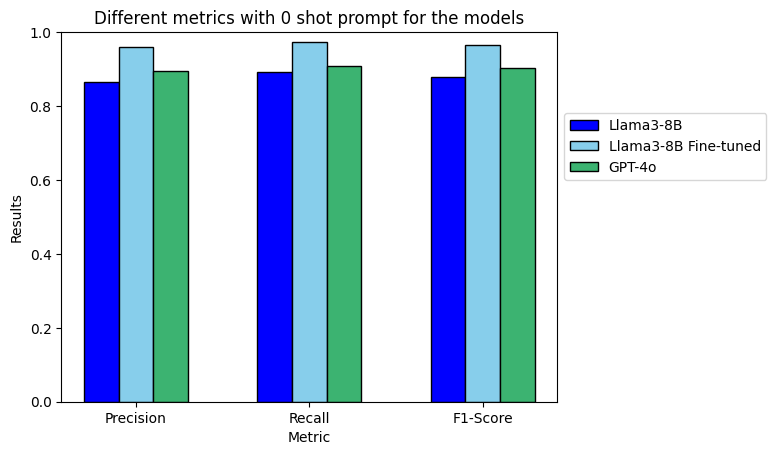
For the zero-shot prompt is possible to see that the best results for all the metrics are the ones obtained when using the fine-tuned model. This is something expected since the fine-tuned model was specifically fine-tuned for this task.
Show code cell source
# set width of bar
barWidth = 0.2
fig = plt.subplots()

plt_data = {}
for index, model in enumerate(plt_models):
    plt_data[model] = metrics_1_shot[index]

# Set position of bar on X axis
br1 = np.arange(len(metrics_1_shot[0]))
br2 = [x + barWidth for x in br1]
br3 = [x + barWidth for x in br2]

# Make the plot
plt.bar(
    br1,
    metrics_1_shot[0],
    color="b",
    width=barWidth,
    edgecolor="black",
    label=plt_models[0],
)
plt.bar(
    br2,
    metrics_1_shot[1],
    color="skyblue",
    width=barWidth,
    edgecolor="black",
    label=plt_models[1],
)
plt.bar(
    br3,
    metrics_1_shot[2],
    color="mediumseagreen",
    width=barWidth,
    edgecolor="black",
    label=plt_models[2],
)

# Adding Xticks
plt.xlabel("Metric")
plt.ylabel("Results")
plt.xticks([r + barWidth for r in range(len(metrics_1_shot[0]))], plt_metrics)
plt.ylim(0, 1)
plt.title("Different metrics with 1-shot prompt for the models")

plt.legend(bbox_to_anchor=(1, 0.8))
# plt.savefig("bars1.png")
plt.show()
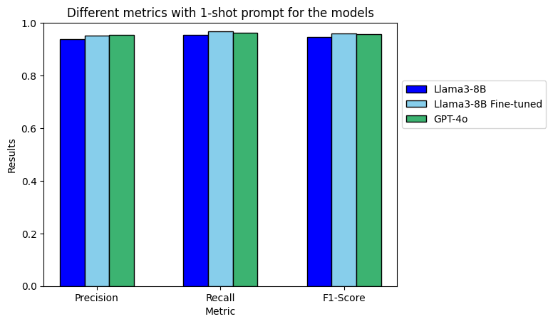
When using the one-shot prompt it is possible to see that the results are slightly better for the closed-source model and for the fine-tuned model.
As pointed above, the fact that the fine-tuned model do not improve the other models is because the fine-tuned model is seeing a format that is not the one that saw during training. Because of that, and having these results to prove it, we recommend avoiding the use of few-shot prompts with fine-tuned models.
Show code cell source
# Organize the results for easy plotting
results = {}

results["llama_results"] = results_llama
results["openai_results"] = results_openai
results["sft_results"] = results_sft

metrics_ = []

for model in models:
    tmp_0 = []
    tmp_1 = []
    for metric in metrics:
        tmp_0.append(results[model + "_results"]["0-shot"][metric])
        tmp_1.append(results[model + "_results"]["1-shot"][metric])
    metrics_.append(tmp_0)
    metrics_.append(tmp_1)

# set width of bar
barWidth = 0.15
fig = plt.subplots()

plt_models = [
    "Llama3-8B 0-shot",
    "Llama3-8B 1-shot",
    "Llama3-8B Fine-tuned 0-shot",
    "Llama3-8B Fine-tuned 1-shot",
    "GPT-4o 0-shot",
    "GPT-4o 1-shot",
]
plt_metrics = ["Precision", "Recall", "F1-Score"]
plt_data = {}
for index, model in enumerate(plt_models):
    plt_data[model] = metrics_[index]

# Set position of bar on X axis
br1 = np.arange(len(metrics_[0]))
br2 = [x + barWidth for x in br1]
br3 = [x + barWidth for x in br2]
br4 = [x + barWidth for x in br3]
br5 = [x + barWidth for x in br4]
br6 = [x + barWidth for x in br5]

# Make the plot
plt.bar(
    br1,
    metrics_[0],
    color="blue",
    width=barWidth,
    edgecolor="black",
    label=plt_models[0],
)
plt.bar(
    br2,
    metrics_[1],
    color="darkblue",
    width=barWidth,
    edgecolor="black",
    label=plt_models[1],
)
plt.bar(
    br3,
    metrics_[2],
    color="lightskyblue",
    width=barWidth,
    edgecolor="black",
    label=plt_models[2],
)
plt.bar(
    br4,
    metrics_[3],
    color="deepskyblue",
    width=barWidth,
    edgecolor="black",
    label=plt_models[3],
)
plt.bar(
    br5,
    metrics_[4],
    color="springgreen",
    width=barWidth,
    edgecolor="black",
    label=plt_models[4],
)
plt.bar(
    br6,
    metrics_[5],
    color="seagreen",
    width=barWidth,
    edgecolor="black",
    label=plt_models[5],
)

# Adding Xticks
plt.xlabel("Metric")
plt.ylabel("Results")
plt.xticks([r + 2.5 * barWidth for r in range(len(metrics_[0]))], plt_metrics)
plt.ylim(0, 1)
plt.title("Different metrics using both prompts for the models")
plt.legend(bbox_to_anchor=(1, 0.8))

# plt.savefig("another.png")
plt.show()
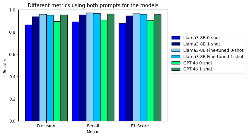
When comparing all the results, it can be clearly seen that the zero-shot fine-tuned model gives the best results overall, with an F\(_1\)-score exceeding 0.95.
Additionally, it is evident that the one-shot prompt yields better results for the not fine-tuned models compared to the zero-shot prompt.
It is also important to highlight the underwhelming results of the fine-tuned model when using the one-shot prompt. This is due to the fact that during the fine-tuning process, the model becomes highly adapted to a specific format, which is disrupted when using the one-shot prompt. Typically, few-shot prompts are not used with the fine-tuned model for this reason.
Lastly, it is crucial to acknowledge that the small differences observed may be attributed to the evaluation method. The BERTScore method measures token-by-token similarity, which may not be very reliable when applied to a JSON schema containing numerous curly brackets and other schema-related tokens. For more reliable evaluations, please refer to the evaluations notebook.
4.7. References#
Qianxiang Ai, Fanwang Meng, Jiale Shi, Brenden Pelkie, and Connor W. Coley. Extracting structured data from organic synthesis procedures using a fine-tuned large language model. ChemRxiv, 2024. doi:10.26434/chemrxiv-2024-979fz.
Tim Dettmers, Mike Lewis, Sam Shleifer, and Luke Zettlemoyer. 8-bit optimizers via block-wise quantization. 2022. arXiv:2110.02861.
Tim Dettmers, Artidoro Pagnoni, Ari Holtzman, and Luke Zettlemoyer. Qlora: efficient finetuning of quantized llms. 2023. arXiv:2305.14314.
Subbarao Kambhampati, Karthik Valmeekam, Lin Guan, Mudit Verma, Kaya Stechly, Siddhant Bhambri, Lucas Saldyt, and Anil Murthy. Llms can't plan, but can help planning in llm-modulo frameworks. 2024. URL: https://arxiv.org/abs/2402.01817, arXiv:2402.01817.
Ilya Loshchilov and Frank Hutter. Decoupled weight decay regularization. 2019. arXiv:1711.05101.
Victor Sanh, Lysandre Debut, Julien Chaumond, and Thomas Wolf. Distilbert, a distilled version of bert: smaller, faster, cheaper and lighter. 2020. arXiv:1910.01108.
Zhengyan Shi, Adam X. Yang, Bin Wu, Laurence Aitchison, Emine Yilmaz, and Aldo Lipani. Instruction tuning with loss over instructions. 2024. arXiv:2405.14394.
Kaya Stechly, Karthik Valmeekam, and Subbarao Kambhampati. On the self-verification limitations of large language models on reasoning and planning tasks. 2024. URL: https://arxiv.org/abs/2402.08115, arXiv:2402.08115.
Tianyi Zhang, Varsha Kishore, Felix Wu, Kilian Q. Weinberger, and Yoav Artzi. Bertscore: evaluating text generation with bert. 2020. arXiv:1904.09675.